- Issues I have faced on my Ubuntu (Linux) system, and their solutions: melwynsubuntuissues.blogspot.com
- My Project Euler solutions database
- My YouTube channel
- My GitHub page
- C Scale, chords, and the 'Mary had a little lamb' song synthetically generated using math: View the GitHub repository
- XS-XML – An extra-small, single-file, portable XML parser and compiler library, written in C as well as in JavaScript: View the GitHub repository
- PyConPTY – A Python-based interface for the ConPTY (Windows Pseudo-console) API: View the PyPI package and View the GitHub repository
- Moment of Area (MoI2) Program – Calculate second moment of inertia (moment of area) from DXF shapes or CSV datapoints using Python: View the GitHub repository
-


This information is about building Synfig directly from its source code.
General information regarding this has been posted by Synfig at this link.
But, that does not suffice, as I have encountered a number of problems while building it on my Windows 10 computer system.
So I put in the effort and figured out a way to successfully build and install it. The following steps will hopefully make your life easier.
- Before you begin, you will first need to download the
MSYS2application from this website, and follow the instructions as given on that website. - Next, launch the
MSYS2 MINGW64application (it's a special command window). If you have a 32-bit computer (most have 64-bit these days), then you might have MINGW32 instead; so, launch that application. Furthermore, (if you have a 32-bit computer) any references to 64-bit in any commands that follow must be replaced with its 32-bit-equivalent, wherever required. - Next, download the source code zip file from this link. Move the zip file to a location of your choice, and then unzip (extract here) the zip file. Enter that folder, (e.g.: synfig-1.5.3) and copy the folder path (Alt + d followed by Ctrl + c).
- In the command window, type cd following by a space, and then paste the copied path and then hit enter.
For instructional purpose, let's assume the folder we're currently in is:synfig-1.5.3 -
Replace the MLT library version in various files from
7.2.0to the latest version. (in my case, it was7.34.1) This version can be obtained by checking out this link.
File path Line number synfig-1.5.3/autobuild/msys2/build_mlt.sh 7 synfig-1.5.3/2-build-cmake.sh 13 synfig-1.5.3/autobuild/synfigstudio-release.sh 45 synfig-1.5.3/cmake/InstallMSYS2.cmake 99 synfig-1.5.3/cmake/InstallMSYS2.cmake 109 synfig-1.5.3/autobuild/build.sh 93
- Open
synfig-1.5.3/autobuild/msys2/build_mlt.sh. On line number 28 (cmake -G"Ninja"...), append the following before the double-dots ('..'):-DJACK_LIBRARY=/mingw64/lib/libjack.dll.a -DCMAKE_PREFIX_PATH=/mingw64 - Using the old Movit library in Synfig causes build error, so let's build it from source.
- Download the latest Movit library file from movit.sesse.net (the latest version is 1.7.2 in tar.gz format as of December 2025). Unzip the zip file in a folder of your choice, and then enter that folder. For instructional purpose, the folder name is:
movit-1.7.2. Copy this folder path. -
In the command window:
- type cd following by a space, and then paste the copied path and then hit enter
- type pacman -S mingw-w64-x86_64-eigen3 and then hit enter
- type CXXFLAGS="-fPIC" ./autogen.sh and then hit enter
- type ./configure --prefix=/mingw64 and then hit enter
-
A few source code amendments:
- Open
movit-1.7.2/Makefile.in, and then replace the whole line number 24 withCXXFLAGS=-Wall @CXXFLAGS@ -fvisibility-inlines-hidden -I$(GTEST_DIR)/include @Eigen3_CFLAGS@ @epoxy_CFLAGS@ @FFTW3_CFLAGS@ @benchmark_CFLAGS@. - Open
movit-1.7.2/effect_chain.cpp, and then replace(long)with(long long). There should be 5 such occurences to replace throughout the file. - Open
movit-1.7.2/fft_convolution_effect.cpp, and then add the following code below the #include pre-processor directives (at around line number 14):
#ifdef __MINGW64__
#define ffs __builtin_ffs
#endif
- Open
- In the command window, type make libmovit.la install and then hit enter
-
In the command window:
- type pacman -S mingw-w64-x86_64-libebur128 mingw-w64-x86_64-qt6-base mingw-w64-x86_64-qt6-declarative mingw-w64-x86_64-qt6-svg mingw-w64-x86_64-qt6-5compat mingw-w64-x86_64-jack2 mingw-w64-x86_64-rtaudio mingw-w64-x86_64-rubberband mingw-w64-x86_64-sox mingw-w64-clang-x86_64-clang mingw-w64-clang-x86_64-clang-tools-extra and then hit enter
- type pacman -S --needed base-devel mingw-w64-x86_64-gcc mingw-w64-x86_64-swig and then hit enter
- type pacman -S --needed gettext gettext-devel and then hit enter
-
In the command window:
- type cp -f C:/msys64/tmp/mlt-7.34.1/build/src/modules/jackrack/mltjackrack_export.h C:/msys64/tmp/mlt-7.34.1/src/modules/jackrack/mltjackrack_export.h and then hit enter
- type cp -f C:/msys64/tmp/mlt-7.34.1/build/src/modules/jackrack/mltladspa_export.h C:/msys64/tmp/mlt-7.34.1/src/modules/jackrack/mltladspa_export.h and then hit enter
- type ln -s /mingw64/lib/libjack64.dll.a /mingw64/lib/libjack.dll.a and then hit enter
- Copy the folder path for the folder
synfig-1.5.3 -
In the command window:
- type cd following by a space, and then paste the copied path and then hit enter
- type ./1-setup-windows-msys2.sh and then hit enter
-
There is a bug in the
intltool-updateprogram that fails the Synfig build.
I have reported this to Ubuntu, and the bug report can be found at this link.
OpenC:/msys64/usr/bin/intltool-update, and on line numbers 628 through 631, replace this:
$srcdir =~ s#^../##;
$dummy =~ s#^$srcdir/../##;
$dummy =~ s#^$srcdir/##;
$dummy =~ s#_build/##;
with this:
$srcdir =~ s#^\Q../\E##;
$dummy =~ s#^\Q$srcdir/../\E##;
$dummy =~ s#^\Q$srcdir/\E##;
$dummy =~ s#_build/##; - In the command window, type ./2-build-debug.sh all full and hit enter (be patient as this process takes a while)
All done!

Algebraic Geometry Computational Geometry C++
I took the initiative to solve the intersection problem to resolve the LibreCAD issue #1459, titled
'Elipse center with
3 points causes freeze when choosing second point'. Looking into the source code,
I came upon an unknown author's TODO comment with regards to another LibreCAD issue #484, titled
'Circles,
the "Snap Intersection" does not work for large coordinates'.
The comment basically stresses the need for an improved conics intersection solver.
This would make redundant other specific solvers for calculating intersections between (any two of)
circles, ellipses, arcs, etc.
The problem was that the solution would fail in certain cases, which happens because
the quartic solver returns no solutions, implying that the solutions lie in the complex plane. By means of simple
observation, it could easily be verified that such an inference is patently incorrect. The problem, by my deduction,
was due to incorrect (or incomplete) conversion of two conic equations into a single, univariate quartic equation.
Furthermore, I did not think about this earlier, but it turns out that this concept can also be applied in the field of
space dynamics to estimate where two astronomical bodies or satellites (in their respective trajectories (or orbits)),
would (or could) eventually meet.
Two dimensional (2D) conic sections are contours generated as a result of a three dimensional (3D) cone and a two dimensional (2D) plane intersecting each other. Conic sections are co-planar on the intersecting plane. Specific conic sections include ellipses, circles (specific case of ellipses), parabolas, and hyperbolas.
The equation for a generic conic section is as follows : \(C = ax^2 + bxy + cy^2 + dx + ey + f = 0\)
The intersection points of any two given conic sections are obtained by solving their simultaneous equations :
(Note that the term \(e\) is an arbitrary coefficient, and not Euler's number.)
\[C_1 = a_1x^2 + b_1xy + c_1y^2 + d_1x + e_1y + f_1 = 0\] \[C_2 = a_2x^2 + b_2xy + c_2y^2 + d_2x + e_2y + f_2 = 0\]
Let us consider two ellipses (just for the purpose of understanding intersections; the solution to the above generic problem will remain generic).
The six possible cases of solutions are as follows:
| Sr. No. | Case | Illustration |
|---|---|---|
| 1. | No intersection | |
| 2.A. | One intersection | |
| 2.B. | One intersection | |
| 3. | Two intersections | |
| 4. | Three intersections | |
| 5. | Four intersections | |
| 6. | Infinite intersections (Coincidental) |
To begin solving, let us first create re-arranged forms of the above equations ( by setting aside the \(y^2\) term ) : \[Y_1^2 = y^2 = {{-a_1x^2 - b_1xy - d_1x - e_1y - f_1} \over {c_1}} = -{{a_1x^2 + b_1xy + d_1x + e_1y + f_1} \over {c_1}}\] \[Y_2^2 = y^2 = {{-a_2x^2 - b_2xy - d_2x - e_2y - f_2} \over {c_2}} = -{{a_2x^2 + b_2xy + d_2x + e_2y + f_2} \over {c_2}}\]
Clearing the fractions, and then simplifying, \[c_2(a_1x^2 + b_1xy + d_1x + e_1y + f_1) = c_1(a_2x^2 + b_2xy + d_2x + e_2y + f_2)\] \[a_1c_2x^2 + b_1c_2xy + c_2d_1x + c_2e_1y + c_2f_1) = a_2c_1x^2 + b_2c_1xy + c_1d_2x + c_1e_2y + c_1f_2\]
Transposing all RHS terms to LHS, and then factoring, \[(a_1c_2 - a_2c_1)x^2 + (b_1c_2 - b_2c_1)xy + (d_1c_2 - d_2c_1)x + (e_1c_2 - e_2c_1)y + (f_1c_2 - f_2c_1) = 0\]
Rearranging to solve for \(y\), \[y = {{-(a_1c_2 - a_2c_1)x^2 - (d_1c_2 - d_2c_1)x - (f_1c_2 - f_2c_1)} \over {(b_1c_2 - b_2c_1)x + (e_1c_2 - e_2c_1)}} = -{{(a_1c_2 - a_2c_1)x^2 + (d_1c_2 - d_2c_1)x + (f_1c_2 - f_2c_1)} \over {(b_1c_2 - b_2c_1)x + (e_1c_2 - e_2c_1)}}\]
Simplifying the terms, \[y = {{y_{numerator}} \over {y_{denominator}}} = {{y_n} \over {y_d}} = {{a_2c_1x^2 - a_1c_2x^2 + d_2c_1x - d_1c_2x + f_2c_1 - f_1c_2} \over {b_1c_2x - b_2c_1x + e_1c_2 - e_2c_1}}\] \[y^2 = {{y_n^2} \over {y_d^2}}\]
Upon simplifying the squares, and then factoring, we get the following equations.
\[\eqalign{y_n^2 &= (a_1^2c_2^2 + a_2^2c_1^2 - 2a_1a_2c_1c_2) \space x^4 \cr &+ (2a_1c_2^2d_1 + 2a_2c_1^2d_2 - 2a_1c_1c_2d_2 - 2a_2c_1c_2d_1) \space x^3 \cr &+ (2a_1c_2^2f_1 + 2a_2c_1^2f_2 + c_1^2d_2^2 + c_2^2d_1^2 - 2a_1c_1c_2f_2 - 2a_2c_1c_2f_1 - 2c_1c_2d_1d_2) \space x^2 \cr &+ (2c_1^2d_2f_2 + 2c_2^2d_1f_1 - 2c_1c_2d_1f_2 - 2c_1c_2d_2f_1) \space x \cr &+ (c_1^2f_2^2 + c_2^2f_1^2 - 2c_1c_2f_1f_2)}\]
\[\eqalign{y_d^2 &= (b_1^2c_2^2 + b_2^2c_1^2 - 2b_1b_2c_1c_2) \space x^2 \cr &+ (2b_1c_2^2e_1 + 2b_2c_1^2e_2 - 2b_1c_1c_2e_2 - 2b_2c_1c_2e_1) \space x \cr &+ (c_1^2e_2^2 + c_2^2e_1^2 - 2c_1c_2e_1e_2)}\]
Substituting the \(y_n\) and \(y_d\) terms into one of the conic sections, say, \(C_1\), we get the following equation. \[C_1 = a_1x^2 + b_1x{{y_n} \over {y_d}} + c_1{{y_n^2} \over {y_d^2}} + d_1x + e_1{{y_n} \over {y_d}} + f_1 = 0\]
Upon clearing the fractions, we get the following equation. \[C_1 = a_1x^2y_d^2 + b_1xy_ny_d + c_1y_n^2 + d_1xy_d^2 + e_1y_ny_d + f_1y_d^2 = 0\]
Upon factoring, we get the following equation. \[C_1 = c_1y_n^2 + (b_1x + e_1)y_ny_d + (a_1x^2 + d_1x + f_1)y_d^2 = 0\]
Upon expanding the \(y_n\) and \(y_d\) terms, we get the following equation. \[\eqalign{C_1 &= (a_1^2c_1c_2^2 + a_2^2c_1^3 - 2a_1a_2c_1^2c_2) \space x^4 \cr &+ (2a_1c_1c_2^2d_1 + 2a_2c_1^3d_2 - 2a_1c_1^2c_2d_2 - 2a_2c_1^2c_2d_1) \space x^3 \cr &+ (2a_1c_1c_2^2f_1 + 2a_2c_1^3f_2 + c_1^3d_2^2 + c_1c_2^2d_1^2 - 2a_1c_1^2c_2f_2 - 2a_2c_1^2c_2f_1 - 2c_1^2c_2d_1d_2) \space x^2 \cr &+ (2c_1^3d_2f_2 + 2c_1c_2^2d_1f_1 - 2c_1^2c_2d_1f_2 - 2c_1^2c_2d_2f_1) \space x \cr &+ (c_1c_2^2f_1^2 + c_1^3f_2^2 - 2c_1^2c_2f_1f_2) \cr \cr &+ (a_1b_1b_2c_1c_2 + a_2b_1^2c_1c_2 - a_1b_1^2c_2^2 - a_2b_1b_2c_1^2) \space x^4 \cr &+ (a_1b_1c_1c_2e_2 + a_1b_2c_1c_2e_1 + 2a_2b_1c_1c_2e_1 + b_1^2c_1c_2d_2 + b_1b_2c_1c_2d_1 - 2a_1b_1c_2^2e_1 - a_2b_1c_1^2e_2 - a_2b_2c_1^2e_1 - b_1^2c_2^2d_1 - b_1b_2c_1^2d_2) \space x^3 \cr &+ (a_1c_1c_2e_1e_2 + a_2c_1c_2e_1^2 + b_1b_2c_1c_2f_1 + b_1c_1c_2d_1e_2 + 2b_1c_1c_2d_2e_1 + b_1^2c_1c_2f_2 + b_2c_1c_2d_1e_1 \cr & \space \space \space \space \space \space \space \space \space \space \space \space - a_1c_2^2e_1^2 - a_2c_1^2e_1e_2 - b_1b_2c_1^2f_2 - b_1c_1^2d_2e_2 - 2b_1c_2^2d_1e_1 - b_1^2c_2^2f_1 - b_2c_1^2d_2e_1) \space x^2 \cr &+ (2b_1c_1c_2e_1f_2 + b_1c_1c_2e_2f_1 + b_2c_1c_2e_1f_1 + c_1c_2d_1e_1e_2 + c_1c_2d_2e_1^2 - b_1c_1^2e_2f_2 - 2b_1c_2^2e_1f_1 - b_2c_1^2e_1f_2 - c_1^2d_2e_1e_2 - c_2^2d_1e_1^2) \space x \cr &+ (c_1c_2e_1^2f_2 + c_1c_2e_1e_2f_1 - c_1^2e_1e_2f_2 - c_2^2e_1^2f_1) \cr \cr &+ (a_1b_1^2c_2^2 + a_1b_2^2c_1^2 - 2a_1b_1b_2c_1c_2) \space x^4 \cr &+ (2a_1b_1c_2^2e_1 + 2a_1b_2c_1^2e_2 + b_1^2c_2^2d_1 + b_2^2c_1^2d_1 - 2a_1b_1c_1c_2e_2 - 2a_1b_2c_1c_2e_1 - 2b_1b_2c_1c_2d_1) \space x^3 \cr &+ (a_1c_1^2e_2^2 + a_1c_2^2e_1^2 + b_1^2c_2^2f_1 + b_2^2c_1^2f_1 + 2b_1c_2^2d_1e_1 + 2b_2c_1^2d_1e_2 - 2a_1c_1c_2e_1e_2 - 2b_1b_2c_1c_2f_1 - 2b_1c_1c_2d_1e_2 - 2b_2c_1c_2d_1e_1) \space x^2 \cr &+ (c_1^2d_1e_2^2 + c_2^2d_1e_1^2 + 2b_1c_2^2e_1f_1 + 2b_2c_1^2e_2f_1 - 2b_1c_1c_2e_2f_1 - 2b_2c_1c_2e_1f_1 - 2c_1c_2d_1e_1e_2) \space x \cr &+ (c_1^2e_2^2f_1 + c_2^2e_1^2f_1 - 2c_1c_2e_1e_2f_1) \cr \cr &= 0}\]
Upon factoring the \(x^n\) terms, we get the following equation of the form \(Ax^4 + Bx^3 + Cx^2 + Dx + K = 0\),
where \(A, B, C,\) and \(D\) are coefficients, and \(K\) is a constant. \[\eqalign{& \space (a_1^2c_1c_2^2 + a_2^2c_1^3 - 2a_1a_2c_1^2c_2 + a_2b_1^2c_1c_2 - a_2b_1b_2c_1^2 + a_1b_2^2c_1^2 - a_1b_1b_2c_1c_2) \space x^4 \cr \cr &+ (2a_1c_1c_2^2d_1 + 2a_2c_1^3d_2 - 2a_1c_1^2c_2d_2 - 2a_2c_1^2c_2d_1 \cr & \space \space \space \space \space + 2a_2b_1c_1c_2e_1 + b_1^2c_1c_2d_2 - a_2b_1c_1^2e_2 - a_2b_2c_1^2e_1 - b_1b_2c_1^2d_2 \cr & \space \space \space \space \space + 2a_1b_2c_1^2e_2 + b_2^2c_1^2d_1 - a_1b_1c_1c_2e_2 - a_1b_2c_1c_2e_1 - b_1b_2c_1c_2d_1) \space x^3 \cr \cr &+ (2a_1c_1c_2^2f_1 + 2a_2c_1^3f_2 + c_1^3d_2^2 + c_1c_2^2d_1^2 - 2a_1c_1^2c_2f_2 - 2a_2c_1^2c_2f_1 - 2c_1^2c_2d_1d_2 \cr & \space \space \space \space \space + a_2c_1c_2e_1^2 + 2b_1c_1c_2d_2e_1 + b_1^2c_1c_2f_2 - a_2c_1^2e_1e_2 - b_1b_2c_1^2f_2 - b_1c_1^2d_2e_2 - b_2c_1^2d_2e_1 \cr & \space \space \space \space \space + a_1c_1^2e_2^2 + b_2^2c_1^2f_1 + 2b_2c_1^2d_1e_2 - a_1c_1c_2e_1e_2 - b_1b_2c_1c_2f_1 - b_1c_1c_2d_1e_2 - b_2c_1c_2d_1e_1) \space x^2 \cr \cr &+ (2c_1^3d_2f_2 + 2c_1c_2^2d_1f_1 - 2c_1^2c_2d_1f_2 - 2c_1^2c_2d_2f_1 \cr & \space \space \space \space \space + 2b_1c_1c_2e_1f_2 + c_1c_2d_2e_1^2 - b_1c_1^2e_2f_2 - b_2c_1^2e_1f_2 - c_1^2d_2e_1e_2 \cr & \space \space \space \space \space + c_1^2d_1e_2^2 + 2b_2c_1^2e_2f_1 - b_1c_1c_2e_2f_1 - b_2c_1c_2e_1f_1 - c_1c_2d_1e_1e_2) \space x \cr \cr &+ (c_1c_2^2f_1^2 + c_1^3f_2^2 - 2c_1^2c_2f_1f_2 + c_1c_2e_1^2f_2 - c_1^2e_1e_2f_2 + c_1^2e_2^2f_1 - c_1c_2e_1e_2f_1) \cr \cr &= 0}\]
This is a quartic (fourth degree) equation. The intersection abscissae (x-coordinates) are the characteristic roots of this equation. A quartic equation may be solved using several methods, though the methods are categorised as either analytic or iterative. Popular examples in the two categories are the 'Ferrari's method' and the 'Newton–Raphson method' .
Care has to be taken to ensure that only solutions in the Real Domain \(( f(x) \in {\mathbb{R}} )\) are stored, and solution in the Complex Domain \(( f(x) \in {\mathbb{C}} )\) are discarded/ignored. Also, care has to be taken to ensure that there is sufficient precision while performing mathematical operations. Relying on float and double for precision-based applications is a folly.
View its source code
Algebraic Geometry
- \((a_1 \neq 0) \land (a_2 \neq 0)\)
- \((b_1 \neq 0) \land (b_2 \neq 0)\)
- \((a_1b_2 \neq a_2b_1)\)
Algebraic Geometry
- \(D \neq 0\)
The \(D\) terms are determinants, and they are defined as follows. \[\eqalign{ D &= \begin{vmatrix} a_1 & b_1 & c_1 \\ a_2 & b_2 & c_2 \\ a_3 & b_3 & c_3 \end{vmatrix} \cr &= a_1(b_2c_3 - b_3c_2) - b_1(a_2c_3 - a_3c_2) + c_1(a_2b_3 - a_3b_2) \cr &= a_1b_2c_3 - a_1b_3c_2 - a_2b_1c_3 + a_3b_1c_2 + a_2b_3c_1 - a_3b_2c_1 \cr \cr D_x &= \begin{vmatrix} -d_1 & b_1 & c_1 \\ -d_2 & b_2 & c_2 \\ -d_3 & b_3 & c_3 \end{vmatrix} \cr &= -d_1(b_2c_3 - b_3c_2) - b_1(-c_3d_2 + c_2d_3) + c_1(-b_3d_2 + b_2d_3) \cr &= b_1c_3d_2 - b_1c_2d_3 + b_2c_1d_3 - b_2c_3d_1 + b_3c_2d_1 - b_3c_1d_2 \cr \cr D_y &= \begin{vmatrix} a_1 & -d_1 & c_1 \\ a_2 & -d_2 & c_2 \\ a_3 & -d_3 & c_3 \end{vmatrix} \cr &= a_1(-c_3d_2 + c_2d_3) + d_1(a_2c_3 - a_3c_2) + c_1(-a_2d_3 + a_3d_2) \cr &= a_1c_2d_3 - a_1c_3d_2 + a_2c_3d_1 - a_2c_1d_3 + a_3c_1d_2 - a_3c_2d_1 \cr \cr D_z &= \begin{vmatrix} a_1 & b_1 & -d_1 \\ a_2 & b_2 & -d_2 \\ a_3 & b_3 & -d_3 \end{vmatrix} \cr &= a_1(-b_2d_3 + b_3d_2) - b_1(-a_2d_3 + a_3d_2) - d_1(a_2b_3 - a_3b_2) \cr &= a_1b_3d_2 - a_1b_2d_3 + a_2b_1d_3 - a_2b_3d_1 + a_3b_2d_1 - a_3b_1d_2 }\]
Subject to the following conditions:
- \(D_{i, *} \neq 0\)
- \(D_{*, j} \neq 0\)
- \(D_{1, *} \neq D_{2, *}\)
- \(D_{1, *} \neq D_{3, *}\)
- \(D_{2, *} \neq D_{3, *}\)
- \(D_{*, 1} \neq D_{*, 2}\)
- \(D_{*, 1} \neq D_{*, 3}\)
- \(D_{*, 2} \neq D_{*, 3}\)
Algebraic Geometry
FIGURE: \( \space \space k = 1 \space \space \) produces a line.
FIGURE: \( \space \space k = 2 \space \space \) produces a circle.
FIGURE: \( \space \space k = \frac{2}{3} = 0.\dot{6} \approx 0.6667 \space \space \)
produces an astroid.
FIGURE: \( \space \space k \to \infty \space \space \)
produces a square.
NOTE that, with respect to the local origin:
- \(0 < k < 1\) produces a concave curve
- \(k > 1 \qquad \) produces a convex curve
For a rectangle (which is a generic form of a square), or a square (which is a specific form of a rectangle), the resolution of its corners is proportional to the \(k\) value. In the above image, \(k = 1000\) was used; \(k = 100\) leads to slightly rounded corners.
Adding horizontal and vertical translations, \(t_x\) and \(t_y\), respectively, modifies the aforementioned equation as follows. \[\bbox[10px, border: 2px solid black]{(x - t_x)^k + (y - t_y)^k = c^k}\] Positive values translate in the rightward and upward directions, respectively, and negative values translate in the leftward and downward directions, respectively. Next, adding horizontal and vertical scale factors, \(s_x\) and \(s_y\), respectively, modifies the equation independently as follows. \[\bbox[10px, border: 2px solid black]{ \left( \frac {x}{s_x} \right) ^k + \left( \frac {y}{s_y} \right) ^k = c^k}\] The scale factors vary proportionally to the required scaling, in either direction. NOTE that, the arbitrary constant, \(c\), can also act as a scale factor that also varies proportionally to the required scaling; however, it scales equally in the horizontal and vertical axes. So, setting \(s_x = f\) and \(s_y = f\) is the same as setting \(c = f\), where \(f\) is an arbitrary scale factor. Finally, adding rotation, \(\theta\), by applying the two-dimensional rotation matrix, modifies the equation independently as follows. \[{(x \cdot cos(\theta) - y \cdot sin(\theta))^k + (x \cdot sin(\theta) + y \cdot cos(\theta))^k = c^k}\]
In the above equation, the angle, \(\theta\), is in the clockwise direction; for counter-clockwise (anti-clockwise) rotation, simply negate the angle, \(\theta\), as \(-\theta\), thereby modifying the above equation as follows.
\[{(x \cdot cos(\theta) + y \cdot sin(\theta))^k + (y \cdot cos(\theta) - x \cdot sin(\theta))^k = c^k}\]
Now, aggregating the above transformations into a single, all-encompassing equation, we get the following equation.
\[ { \left\{ \frac { \left[ (x - t_x) \cdot cos(\theta) \right] + \left[ (y - t_y) \cdot sin(\theta) \right] } {s_x} \right\} ^ k + \left\{ \frac { \left[ (y - t_y) \cdot cos(\theta) \right] - \left[ (x - t_x) \cdot sin(\theta) \right] } {s_y} \right\} ^ k = c^k}\]
\[ { s_y^k \cdot \left\{ \left[ (x - t_x) \cdot cos(\theta) \right] + \left[ (y - t_y) \cdot sin(\theta) \right] \right\} ^ k + s_x^k \cdot \left\{ \left[ (y - t_y) \cdot cos(\theta) \right] - \left[ (x - t_x) \cdot sin(\theta) \right] \right\} ^ k =c^{k}s_x^{k}s_y^{k}}\]
This final equation can be used to create and transform a generic rectangle. Illustrated below is a two-by-one \( (2 \times 1) \) rectangle, translated rightward and upward by two units each \( (+2, +2) \), and rotated clockwise by forty-five degrees \( \left( -45^{\circ} \space \text{or} \space -\frac{\pi}{4}^c \space \text{or} \space +\frac{7\pi}{4}^c \right) \).
\[ { \left\{ \frac { \left[ (x - 2) \cdot cos \left( - \frac{\pi}{4} \right) \right] + \left[ (y - 2) \cdot sin \left( - \frac{\pi}{4} \right) \right] } {2} \right\} ^ {100} + \left\{ \left[ (y - 2) \cdot cos \left( - \frac{\pi}{4} \right) \right] - \left[ (x - 2) \cdot sin \left( - \frac{\pi}{4} \right) \right] \right\} ^ {100} = 1}\]
\[ { \left[ \space 0.35355 (x - 2) \space - \space 0.35355 (y - 2) \space \right] ^ {100} + \left[ \space 0.7071 (x - 2) \space + \space 0.7071 (y - 2) \space \right] ^ {100} = 1}\]
Computational Geometry
- the contour of the outer (blue) rectangle represents the CAD window's drawable area.
- the contour of the inner (grey) rectangle represents the unprobed area for the auto-pan function.
- the blue strip area is the region where the auto-pan function is supposed to operate.
- \(C (x, y)\) is the centre point of the CAD window's drawable area.
- \(P (x, y)\) is an arbitrary mouse (cursor) position
- \(P (x, y)\) is located within the perimeter of the unprobed area
- \(P (x, y)\) is located outside the perimeter of the CAD window's drawable area
- an imaginary line is drawn connecting point \(C (x, y)\) and point \(P (x, y)\).
- Point \(U (x, y)\) is the CAD drawable area's upper-right corner.
Considering the two points \(C\) and \(P\), a right triangle can be formed, as illustrated below.
Note that all angles follow the counter-clockwise (anti-clockwise) direction. Now, extend the vertical line in the above illustrated right triange, such that it cuts the borders of the inner and outer rectangular areas. This is illustrated below, with the term \(L\) denoting lengths.
Let \(\alpha\), a constant, be the CAD drawable area's quarter angle, brought about by the vector, \(\overrightarrow{CU}\). Then, \[\alpha = tan^{-1} \left( \frac {U_y - C_y}{U_x - C_x} \right)\] \[L = \begin{cases} \left| P_y - C_y \right|, & \text{if} \space \space \space \space \space \space \space \space \space \space \space \alpha \lt \theta \leqslant \pi - \alpha \\ \left| P_y - C_y \right|, & \text{if} \space \space \space \space \pi + \alpha \lt \theta \leqslant 2 \pi - \alpha \\ \left| P_x - C_x \right|, & \text{if} \space \space \space \space \pi - \alpha \lt \theta \leqslant \pi + \alpha \\ \left| P_x - C_x \right|, & \text{if} \space \space 2 \pi - \alpha \lt \theta \leqslant \alpha \end{cases}\] \[L_I = \begin{cases} \frac{H_I}{2}, & \text{if} \space \space \space \space \space \space \space \space \space \space \space \alpha \lt \theta \leqslant \pi - \alpha \\ \frac{H_I}{2}, & \text{if} \space \space \space \space \pi + \alpha \lt \theta \leqslant 2 \pi - \alpha \\ \frac{W_I}{2}, & \text{if} \space \space \space \space \pi - \alpha \lt \theta \leqslant \pi + \alpha \\ \frac{W_I}{2}, & \text{if} \space \space 2 \pi - \alpha \lt \theta \leqslant \alpha \end{cases}\] \[L_O = \begin{cases} \frac{H_O}{2}, & \text{if} \space \space \space \space \space \space \space \space \space \space \space \alpha \lt \theta \leqslant \pi - \alpha \\ \frac{H_O}{2}, & \text{if} \space \space \space \space \pi + \alpha \lt \theta \leqslant 2 \pi - \alpha \\ \frac{W_O}{2}, & \text{if} \space \space \space \space \pi - \alpha \lt \theta \leqslant \pi + \alpha \\ \frac{W_O}{2}, & \text{if} \space \space 2 \pi - \alpha \lt \theta \leqslant \alpha \end{cases}\]
The percentage of the mouse (cursor) position with respect to it's minimum and maximum allowable points, \(I\) and \(O\), respectively,
(called the Percentage Factor, or \(PF\)) is calculated as follows. \[PF = \frac {L - L_I} {L_O - L_I}\]
The pan displacement/offset vector, in the polar coordinate system, is \((R, \theta)\), where \(R\), a constant, is the pan offset magnitude.
For auto-panning, the pan operation is periodically repeated. The interval period is inversely proportional to the required speed of the auto-pan operation. The auto-pan timer interval, \(APTI\), is calculated as follows, where \(APTI_{MIN}\) and \(APTI_{MAX}\) are its minimum and maximum constants. \[APTI = APTI_{MIN} + \left[ ( APTI_{MAX} - APTI_{MIN}) \space \cdot \space (1.0 - PF) ) \right]\]
View its source code
Bash (Shell)
View its source code
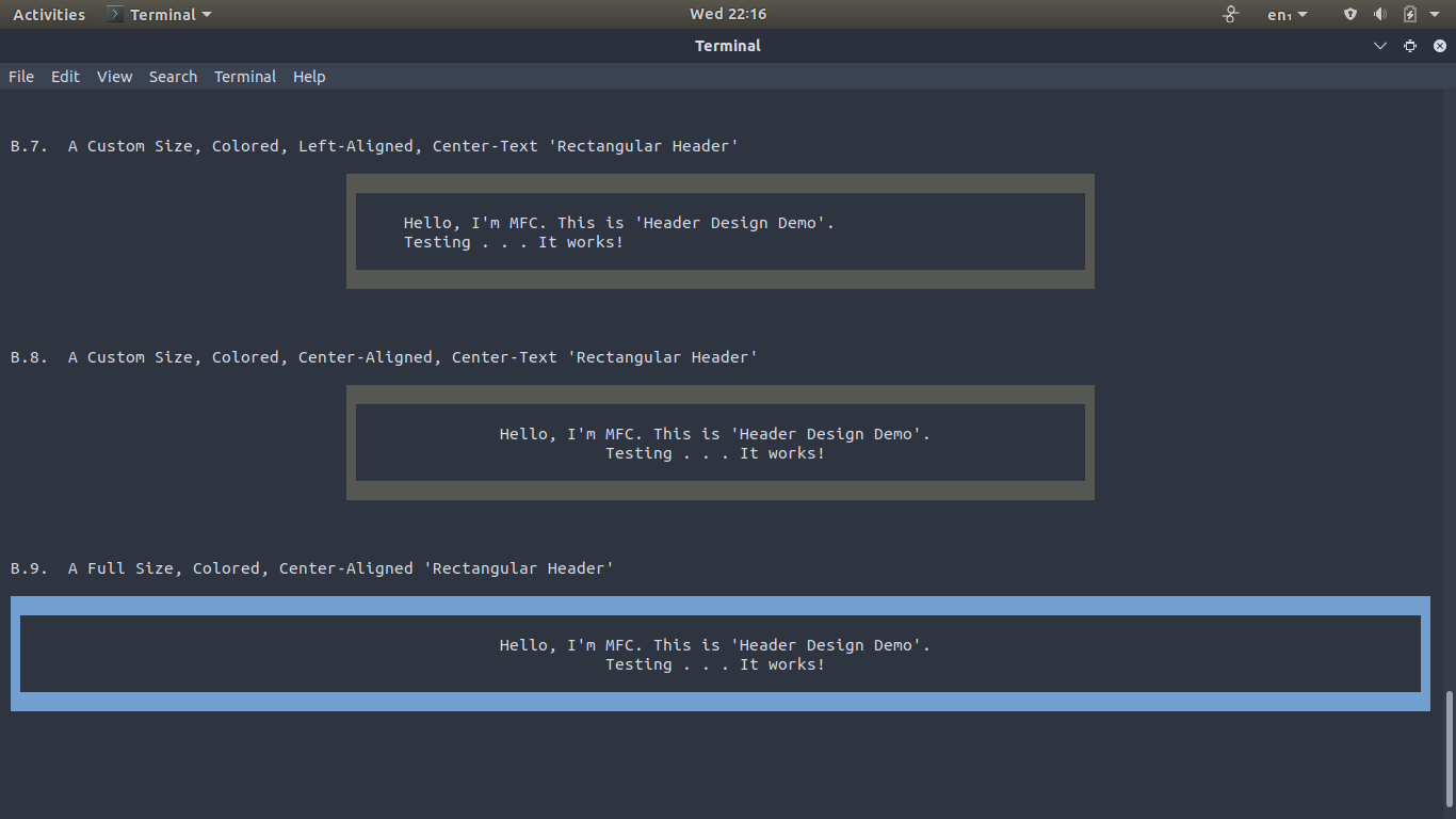
Bash (Shell)
View its source code
Bash (Shell)
View its source code
Bash (Shell)
View its source code