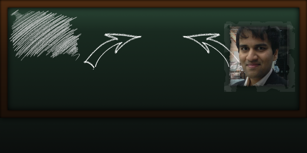
Sorry! No image available at the moment.

MELWYN - FRANCIS - CARLO
Date of Birth	:	30 September, 1996 (24 years)
Location	:	Mumbai, MH, India 🇮🇳
Competitive Exams	:	GRE [ Score : 321/340 ]
Human Languages	:	English, Konkani, Hindi, Marathi, French & German
Fictional Languages	:	Wizadry Spells in Latin & Klingon
Computing Languages	:	C, C++, Bash (Shell), Fortran, Java, JavaScript (JS), Python, Matlab, Scilab, HTML, CSS, PHP, ADA, Assembly Code & Machine Code

The following are my favourite software:

Software name	Purpose
Gedit	Note-taking and developing (all programming languages).
Typora	Diary writing, using rich-text markdown.
Lilypond and Frescobaldi	Composing music, and compiling it into PDF and MIDI formats.
LibreOffice	LibreWriter, LibreCalc, LibreImpress, and LibreBase as substitutes for MS-Word, MS-Excel, and MS-PowerPoint, and MS-Access respectively; LibreDraw for developing custom SVG images.
Audacity	Audio editing.
Kdenlive	Video creation and editing.
FreeCAD	Designing 3D solid models.
Scilab and XCos	Substitutes for MATLAB AND Simulink, respectively.
Freeplane	Drawing mind-maps for brainstorming and planning purposes.
Eclipse Papyrus and Plant UML	UML and SysML Diagrams
Diagrams.net (formerly draw.io) and Dia	Flowcharts and block diagrams.
Android SDK	Develop Android mobile phone applications, using Kotlin.
OpenJDK	Compile and execute Java code.
Gnome Glade/ Gluon SceneBuilder	GUI desktop applications development. Glade is for Linux apps, written in C, using the GTK3 library. SceneBuilder is for cross-platform apps, written in Java, using the JavaFX library.
Apache Superset/ Tableau	Business Intelligence (BI), Data Exploration and Data Visualisation.

.col

⌄

Bi-Conic Sections Intersection Solver
Algebraic Geometry Computational Geometry C++

# 1

I took the initiative to solve the intersection problem to resolve the LibreCAD issue #1459, titled 'Elipse center with 3 points causes freeze when choosing second point' . Looking into the source code, I came upon an unknown author's TODO comment with regards to another LibreCAD issue #484, titled 'Circles, the "Snap Intersection" does not work for large coordinates' . The comment basically stresses the need for an improved conics intersection solver. This would make redundant other specific solvers for calculating intersections between (any two of) circles, ellipses, arcs, etc.

The problem was that the solution would fail in certain cases, which happens because the quartic solver returns no solutions, implying that the solutions lie in the complex plane. By means of simple observation, it could easily be verified that such an inference is patently incorrect. The problem, by my deduction, was due to incorrect (or incomplete) conversion of two conic equations into a single, univariate quartic equation.

Furthermore, I did not think about this earlier, but it turns out that this concept can also be applied in the field of space dynamics to estimate where two astronomical bodies or satellites (in their respective trajectories (or orbits)), would (or could) eventually meet.

Two dimensional (2D) conic sections are contours generated as a result of a three dimensional (3D) cone and a two dimensional (2D) plane intersecting each other. Conic sections are co-planar on the intersecting plane. Specific conic sections include ellipses, circles (specific case of ellipses), parabolas, and hyperbolas.

The equation for a generic conic section is as follows :

C = a x^{2} + b x y + c y^{2} + d x + e y + f = 0

The intersection points of any two given conic sections are obtained by solving their simultaneous equations :
(Note that the term

e

is an arbitrary coefficient, and not Euler's number.)

C_{1} = a_{1} x^{2} + b_{1} x y + c_{1} y^{2} + d_{1} x + e_{1} y + f_{1} = 0

C_{2} = a_{2} x^{2} + b_{2} x y + c_{2} y^{2} + d_{2} x + e_{2} y + f_{2} = 0

Let us consider two ellipses (just for the purpose of understanding intersections; the solution to the above generic problem will remain generic).
The six possible cases of solutions are as follows.

Sr. No.	Case	Illustration
1.	No intersection
2.A.	One intersection
2.B.	One intersection
3.	Two intersections
4.	Three intersections
5.	Four intersections
6.	Infinite intersections (Coincidental)

To begin solving, let us first create re-arranged forms of the above equations ( by setting aside the

y^{2}

term ) :

Y_{1}^{2} = y^{2} = \frac{- a_{1} x^{2} - b_{1} x y - d_{1} x - e_{1} y - f_{1}}{c_{1}} = - \frac{a_{1} x^{2} + b_{1} x y + d_{1} x + e_{1} y + f_{1}}{c_{1}}

Y_{2}^{2} = y^{2} = \frac{- a_{2} x^{2} - b_{2} x y - d_{2} x - e_{2} y - f_{2}}{c_{2}} = - \frac{a_{2} x^{2} + b_{2} x y + d_{2} x + e_{2} y + f_{2}}{c_{2}}

Clearing the fractions, and then simplifying,

c_{2} (a_{1} x^{2} + b_{1} x y + d_{1} x + e_{1} y + f_{1}) = c_{1} (a_{2} x^{2} + b_{2} x y + d_{2} x + e_{2} y + f_{2})

a_{1} c_{2} x^{2} + b_{1} c_{2} x y + c_{2} d_{1} x + c_{2} e_{1} y + c_{2} f_{1}) = a_{2} c_{1} x^{2} + b_{2} c_{1} x y + c_{1} d_{2} x + c_{1} e_{2} y + c_{1} f_{2}

Transposing all RHS terms to LHS, and then factoring,

(a_{1} c_{2} - a_{2} c_{1}) x^{2} + (b_{1} c_{2} - b_{2} c_{1}) x y + (d_{1} c_{2} - d_{2} c_{1}) x + (e_{1} c_{2} - e_{2} c_{1}) y + (f_{1} c_{2} - f_{2} c_{1}) = 0

Rearranging to solve for

y

y = \frac{- (a_{1} c_{2} - a_{2} c_{1}) x^{2} - (d_{1} c_{2} - d_{2} c_{1}) x - (f_{1} c_{2} - f_{2} c_{1})}{(b_{1} c_{2} - b_{2} c_{1}) x + (e_{1} c_{2} - e_{2} c_{1})} = - \frac{(a_{1} c_{2} - a_{2} c_{1}) x^{2} + (d_{1} c_{2} - d_{2} c_{1}) x + (f_{1} c_{2} - f_{2} c_{1})}{(b_{1} c_{2} - b_{2} c_{1}) x + (e_{1} c_{2} - e_{2} c_{1})}

Simplifying the terms,

y = \frac{y_{n u m e r a t o r}}{y_{d e n o m i n a t o r}} = \frac{y_{n}}{y_{d}} = \frac{a_{2} c_{1} x^{2} - a_{1} c_{2} x^{2} + d_{2} c_{1} x - d_{1} c_{2} x + f_{2} c_{1} - f_{1} c_{2}}{b_{1} c_{2} x - b_{2} c_{1} x + e_{1} c_{2} - e_{2} c_{1}}

y^{2} = \frac{y_{n}^{2}}{y_{d}^{2}}

Upon simplifying the squares, and then factoring, we get the following equations.

\begin{aligned} y_{n}^{2} & = (a_{1}^{2} c_{2}^{2} + a_{2}^{2} c_{1}^{2} - 2 a_{1} a_{2} c_{1} c_{2}) x^{4} \\ + (2 a_{1} c_{2}^{2} d_{1} + 2 a_{2} c_{1}^{2} d_{2} - 2 a_{1} c_{1} c_{2} d_{2} - 2 a_{2} c_{1} c_{2} d_{1}) x^{3} \\ + (2 a_{1} c_{2}^{2} f_{1} + 2 a_{2} c_{1}^{2} f_{2} + c_{1}^{2} d_{2}^{2} + c_{2}^{2} d_{1}^{2} - 2 a_{1} c_{1} c_{2} f_{2} - 2 a_{2} c_{1} c_{2} f_{1} - 2 c_{1} c_{2} d_{1} d_{2}) x^{2} \\ + (2 c_{1}^{2} d_{2} f_{2} + 2 c_{2}^{2} d_{1} f_{1} - 2 c_{1} c_{2} d_{1} f_{2} - 2 c_{1} c_{2} d_{2} f_{1}) x \\ + (c_{1}^{2} f_{2}^{2} + c_{2}^{2} f_{1}^{2} - 2 c_{1} c_{2} f_{1} f_{2}) \end{aligned}

\begin{aligned} y_{d}^{2} & = (b_{1}^{2} c_{2}^{2} + b_{2}^{2} c_{1}^{2} - 2 b_{1} b_{2} c_{1} c_{2}) x^{2} \\ + (2 b_{1} c_{2}^{2} e_{1} + 2 b_{2} c_{1}^{2} e_{2} - 2 b_{1} c_{1} c_{2} e_{2} - 2 b_{2} c_{1} c_{2} e_{1}) x \\ + (c_{1}^{2} e_{2}^{2} + c_{2}^{2} e_{1}^{2} - 2 c_{1} c_{2} e_{1} e_{2}) \end{aligned}

Substituting the

y_{n}

and

y_{d}

terms into one of the conic sections, say,

C_{1}

, we get the following equation.

C_{1} = a_{1} x^{2} + b_{1} x \frac{y_{n}}{y_{d}} + c_{1} \frac{y_{n}^{2}}{y_{d}^{2}} + d_{1} x + e_{1} \frac{y_{n}}{y_{d}} + f_{1} = 0

Upon clearing the fractions, we get the following equation.

C_{1} = a_{1} x^{2} y_{d}^{2} + b_{1} x y_{n} y_{d} + c_{1} y_{n}^{2} + d_{1} x y_{d}^{2} + e_{1} y_{n} y_{d} + f_{1} y_{d}^{2} = 0

Upon factoring, we get the following equation.

C_{1} = c_{1} y_{n}^{2} + (b_{1} x + e_{1}) y_{n} y_{d} + (a_{1} x^{2} + d_{1} x + f_{1}) y_{d}^{2} = 0

Upon expanding the

y_{n}

and

y_{d}

terms, we get the following equation.

\begin{aligned} C_{1} & = (a_{1}^{2} c_{1} c_{2}^{2} + a_{2}^{2} c_{1}^{3} - 2 a_{1} a_{2} c_{1}^{2} c_{2}) x^{4} \\ + (2 a_{1} c_{1} c_{2}^{2} d_{1} + 2 a_{2} c_{1}^{3} d_{2} - 2 a_{1} c_{1}^{2} c_{2} d_{2} - 2 a_{2} c_{1}^{2} c_{2} d_{1}) x^{3} \\ + (2 a_{1} c_{1} c_{2}^{2} f_{1} + 2 a_{2} c_{1}^{3} f_{2} + c_{1}^{3} d_{2}^{2} + c_{1} c_{2}^{2} d_{1}^{2} - 2 a_{1} c_{1}^{2} c_{2} f_{2} - 2 a_{2} c_{1}^{2} c_{2} f_{1} - 2 c_{1}^{2} c_{2} d_{1} d_{2}) x^{2} \\ + (2 c_{1}^{3} d_{2} f_{2} + 2 c_{1} c_{2}^{2} d_{1} f_{1} - 2 c_{1}^{2} c_{2} d_{1} f_{2} - 2 c_{1}^{2} c_{2} d_{2} f_{1}) x \\ + (c_{1} c_{2}^{2} f_{1}^{2} + c_{1}^{3} f_{2}^{2} - 2 c_{1}^{2} c_{2} f_{1} f_{2}) \\ + (a_{1} b_{1} b_{2} c_{1} c_{2} + a_{2} b_{1}^{2} c_{1} c_{2} - a_{1} b_{1}^{2} c_{2}^{2} - a_{2} b_{1} b_{2} c_{1}^{2}) x^{4} \\ + (a_{1} b_{1} c_{1} c_{2} e_{2} + a_{1} b_{2} c_{1} c_{2} e_{1} + 2 a_{2} b_{1} c_{1} c_{2} e_{1} + b_{1}^{2} c_{1} c_{2} d_{2} + b_{1} b_{2} c_{1} c_{2} d_{1} - 2 a_{1} b_{1} c_{2}^{2} e_{1} - a_{2} b_{1} c_{1}^{2} e_{2} - a_{2} b_{2} c_{1}^{2} e_{1} - b_{1}^{2} c_{2}^{2} d_{1} - b_{1} b_{2} c_{1}^{2} d_{2}) x^{3} \\ + (a_{1} c_{1} c_{2} e_{1} e_{2} + a_{2} c_{1} c_{2} e_{1}^{2} + b_{1} b_{2} c_{1} c_{2} f_{1} + b_{1} c_{1} c_{2} d_{1} e_{2} + 2 b_{1} c_{1} c_{2} d_{2} e_{1} + b_{1}^{2} c_{1} c_{2} f_{2} + b_{2} c_{1} c_{2} d_{1} e_{1} \\ - a_{1} c_{2}^{2} e_{1}^{2} - a_{2} c_{1}^{2} e_{1} e_{2} - b_{1} b_{2} c_{1}^{2} f_{2} - b_{1} c_{1}^{2} d_{2} e_{2} - 2 b_{1} c_{2}^{2} d_{1} e_{1} - b_{1}^{2} c_{2}^{2} f_{1} - b_{2} c_{1}^{2} d_{2} e_{1}) x^{2} \\ + (2 b_{1} c_{1} c_{2} e_{1} f_{2} + b_{1} c_{1} c_{2} e_{2} f_{1} + b_{2} c_{1} c_{2} e_{1} f_{1} + c_{1} c_{2} d_{1} e_{1} e_{2} + c_{1} c_{2} d_{2} e_{1}^{2} - b_{1} c_{1}^{2} e_{2} f_{2} - 2 b_{1} c_{2}^{2} e_{1} f_{1} - b_{2} c_{1}^{2} e_{1} f_{2} - c_{1}^{2} d_{2} e_{1} e_{2} - c_{2}^{2} d_{1} e_{1}^{2}) x \\ + (c_{1} c_{2} e_{1}^{2} f_{2} + c_{1} c_{2} e_{1} e_{2} f_{1} - c_{1}^{2} e_{1} e_{2} f_{2} - c_{2}^{2} e_{1}^{2} f_{1}) \\ + (a_{1} b_{1}^{2} c_{2}^{2} + a_{1} b_{2}^{2} c_{1}^{2} - 2 a_{1} b_{1} b_{2} c_{1} c_{2}) x^{4} \\ + (2 a_{1} b_{1} c_{2}^{2} e_{1} + 2 a_{1} b_{2} c_{1}^{2} e_{2} + b_{1}^{2} c_{2}^{2} d_{1} + b_{2}^{2} c_{1}^{2} d_{1} - 2 a_{1} b_{1} c_{1} c_{2} e_{2} - 2 a_{1} b_{2} c_{1} c_{2} e_{1} - 2 b_{1} b_{2} c_{1} c_{2} d_{1}) x^{3} \\ + (a_{1} c_{1}^{2} e_{2}^{2} + a_{1} c_{2}^{2} e_{1}^{2} + b_{1}^{2} c_{2}^{2} f_{1} + b_{2}^{2} c_{1}^{2} f_{1} + 2 b_{1} c_{2}^{2} d_{1} e_{1} + 2 b_{2} c_{1}^{2} d_{1} e_{2} - 2 a_{1} c_{1} c_{2} e_{1} e_{2} - 2 b_{1} b_{2} c_{1} c_{2} f_{1} - 2 b_{1} c_{1} c_{2} d_{1} e_{2} - 2 b_{2} c_{1} c_{2} d_{1} e_{1}) x^{2} \\ + (c_{1}^{2} d_{1} e_{2}^{2} + c_{2}^{2} d_{1} e_{1}^{2} + 2 b_{1} c_{2}^{2} e_{1} f_{1} + 2 b_{2} c_{1}^{2} e_{2} f_{1} - 2 b_{1} c_{1} c_{2} e_{2} f_{1} - 2 b_{2} c_{1} c_{2} e_{1} f_{1} - 2 c_{1} c_{2} d_{1} e_{1} e_{2}) x \\ + (c_{1}^{2} e_{2}^{2} f_{1} + c_{2}^{2} e_{1}^{2} f_{1} - 2 c_{1} c_{2} e_{1} e_{2} f_{1}) \\ = 0 \end{aligned}

Upon factoring the

x^{n}

terms, we get the following equation of the form

A x^{4} + B x^{3} + C x^{2} + D x + K = 0

,
where

A, B, C,

and

D

are coefficients, and

K

is a constant.

\begin{aligned} (a_{1}^{2} c_{1} c_{2}^{2} + a_{2}^{2} c_{1}^{3} - 2 a_{1} a_{2} c_{1}^{2} c_{2} + a_{2} b_{1}^{2} c_{1} c_{2} - a_{2} b_{1} b_{2} c_{1}^{2} + a_{1} b_{2}^{2} c_{1}^{2} - a_{1} b_{1} b_{2} c_{1} c_{2}) x^{4} \\ + (2 a_{1} c_{1} c_{2}^{2} d_{1} + 2 a_{2} c_{1}^{3} d_{2} - 2 a_{1} c_{1}^{2} c_{2} d_{2} - 2 a_{2} c_{1}^{2} c_{2} d_{1} \\ + 2 a_{2} b_{1} c_{1} c_{2} e_{1} + b_{1}^{2} c_{1} c_{2} d_{2} - a_{2} b_{1} c_{1}^{2} e_{2} - a_{2} b_{2} c_{1}^{2} e_{1} - b_{1} b_{2} c_{1}^{2} d_{2} \\ + 2 a_{1} b_{2} c_{1}^{2} e_{2} + b_{2}^{2} c_{1}^{2} d_{1} - a_{1} b_{1} c_{1} c_{2} e_{2} - a_{1} b_{2} c_{1} c_{2} e_{1} - b_{1} b_{2} c_{1} c_{2} d_{1}) x^{3} \\ + (2 a_{1} c_{1} c_{2}^{2} f_{1} + 2 a_{2} c_{1}^{3} f_{2} + c_{1}^{3} d_{2}^{2} + c_{1} c_{2}^{2} d_{1}^{2} - 2 a_{1} c_{1}^{2} c_{2} f_{2} - 2 a_{2} c_{1}^{2} c_{2} f_{1} - 2 c_{1}^{2} c_{2} d_{1} d_{2} \\ + a_{2} c_{1} c_{2} e_{1}^{2} + 2 b_{1} c_{1} c_{2} d_{2} e_{1} + b_{1}^{2} c_{1} c_{2} f_{2} - a_{2} c_{1}^{2} e_{1} e_{2} - b_{1} b_{2} c_{1}^{2} f_{2} - b_{1} c_{1}^{2} d_{2} e_{2} - b_{2} c_{1}^{2} d_{2} e_{1} \\ + a_{1} c_{1}^{2} e_{2}^{2} + b_{2}^{2} c_{1}^{2} f_{1} + 2 b_{2} c_{1}^{2} d_{1} e_{2} - a_{1} c_{1} c_{2} e_{1} e_{2} - b_{1} b_{2} c_{1} c_{2} f_{1} - b_{1} c_{1} c_{2} d_{1} e_{2} - b_{2} c_{1} c_{2} d_{1} e_{1}) x^{2} \\ + (2 c_{1}^{3} d_{2} f_{2} + 2 c_{1} c_{2}^{2} d_{1} f_{1} - 2 c_{1}^{2} c_{2} d_{1} f_{2} - 2 c_{1}^{2} c_{2} d_{2} f_{1} \\ + 2 b_{1} c_{1} c_{2} e_{1} f_{2} + c_{1} c_{2} d_{2} e_{1}^{2} - b_{1} c_{1}^{2} e_{2} f_{2} - b_{2} c_{1}^{2} e_{1} f_{2} - c_{1}^{2} d_{2} e_{1} e_{2} \\ + c_{1}^{2} d_{1} e_{2}^{2} + 2 b_{2} c_{1}^{2} e_{2} f_{1} - b_{1} c_{1} c_{2} e_{2} f_{1} - b_{2} c_{1} c_{2} e_{1} f_{1} - c_{1} c_{2} d_{1} e_{1} e_{2}) x \\ + (c_{1} c_{2}^{2} f_{1}^{2} + c_{1}^{3} f_{2}^{2} - 2 c_{1}^{2} c_{2} f_{1} f_{2} + c_{1} c_{2} e_{1}^{2} f_{2} - c_{1}^{2} e_{1} e_{2} f_{2} + c_{1}^{2} e_{2}^{2} f_{1} - c_{1} c_{2} e_{1} e_{2} f_{1}) \\ = 0 \end{aligned}

This is a quartic (fourth degree) equation. The intersection abscissae (x-coordinates) are the characteristic roots of this equation. A quartic equation may be solved using several methods, though the methods are categorised as either analytic or iterative. Popular examples in the two categories are the 'Ferrari's method' and the 'Newton–Raphson method' .

Care has to be taken to ensure that only solutions in the Real Domain

(f (x) \in R)

are stored, and solution in the Complex Domain

(f (x) \in C)

are discarded/ignored. Also, care has to be taken to ensure that there is sufficient precision while performing mathematical operations. Relying on float and double for precision-based applications is a folly.

Visit its Source !

⌄

System of Bi-Linear Simultaneous Equations Solver
Algebraic Geometry

# 2

Consider the following two generic linear equations in two variables:

a_{1} x + b_{1} y + c_{1} = 0

a_{2} x + b_{2} y + c_{2} = 0

Re-arranging to solve for the

y

term in the second equation, we get

y = \frac{- a_{2} x - c_{2}}{b_{2}} = - \frac{a_{2} x + c_{2}}{b_{2}}

Substituting the second equation's

y

term in the first equation, we get

x = \frac{b_{1} c_{2} - b_{2} c_{1}}{a_{1} b_{2} - a_{2} b_{1}}

Similarly, re-arranging to solve for the

x

term in the second equation, we get

y = \frac{- a_{2} x - c_{2}}{b_{2}} = - \frac{a_{2} x + c_{2}}{b_{2}}

And then, substituting the second equation's

x

term in the first equation, we get

y = \frac{a_{1} c_{2} - a_{2} c_{1}}{a_{2} b_{1} - a_{1} b_{2}}

Subject to the following conditions:

$(a_{1} \neq 0) \land (a_{2} \neq 0)$
$(b_{1} \neq 0) \land (b_{2} \neq 0)$
$(a_{1} b_{2} \neq a_{2} b_{1})$

⌄

System of Tri-Linear Simultaneous Equations Solver
Algebraic Geometry

# 3

Consider the following three generic linear equations in three variables:

a_{1} x + b_{1} y + c_{1} z + d_{1} = 0

a_{2} x + b_{2} y + c_{2} z + d_{2} = 0

a_{3} x + b_{3} y + c_{3} z + d_{3} = 0

Using Cramer's rule,

x = \frac{D_{x}}{D}

y = \frac{D_{y}}{D}

z = \frac{D_{z}}{D}

Subject to the following condition:

$D \neq 0$

The

D

terms are determinants, and they are defined as follows.

\begin{aligned} D & = | \begin{array}{c} a_{1} & b_{1} & c_{1} \\ a_{2} & b_{2} & c_{2} \\ a_{3} & b_{3} & c_{3} \end{array} | \\ = a_{1} (b_{2} c_{3} - b_{3} c_{2}) - b_{1} (a_{2} c_{3} - a_{3} c_{2}) + c_{1} (a_{2} b_{3} - a_{3} b_{2}) \\ = a_{1} b_{2} c_{3} - a_{1} b_{3} c_{2} - a_{2} b_{1} c_{3} + a_{3} b_{1} c_{2} + a_{2} b_{3} c_{1} - a_{3} b_{2} c_{1} \\ D_{x} & = | \begin{array}{c} - d_{1} & b_{1} & c_{1} \\ - d_{2} & b_{2} & c_{2} \\ - d_{3} & b_{3} & c_{3} \end{array} | \\ = - d_{1} (b_{2} c_{3} - b_{3} c_{2}) - b_{1} (- c_{3} d_{2} + c_{2} d_{3}) + c_{1} (- b_{3} d_{2} + b_{2} d_{3}) \\ = b_{1} c_{3} d_{2} - b_{1} c_{2} d_{3} + b_{2} c_{1} d_{3} - b_{2} c_{3} d_{1} + b_{3} c_{2} d_{1} - b_{3} c_{1} d_{2} \\ D_{y} & = | \begin{array}{c} a_{1} & - d_{1} & c_{1} \\ a_{2} & - d_{2} & c_{2} \\ a_{3} & - d_{3} & c_{3} \end{array} | \\ = a_{1} (- c_{3} d_{2} + c_{2} d_{3}) + d_{1} (a_{2} c_{3} - a_{3} c_{2}) + c_{1} (- a_{2} d_{3} + a_{3} d_{2}) \\ = a_{1} c_{2} d_{3} - a_{1} c_{3} d_{2} + a_{2} c_{3} d_{1} - a_{2} c_{1} d_{3} + a_{3} c_{1} d_{2} - a_{3} c_{2} d_{1} \\ D_{z} & = | \begin{array}{c} a_{1} & b_{1} & - d_{1} \\ a_{2} & b_{2} & - d_{2} \\ a_{3} & b_{3} & - d_{3} \end{array} | \\ = a_{1} (- b_{2} d_{3} + b_{3} d_{2}) - b_{1} (- a_{2} d_{3} + a_{3} d_{2}) - d_{1} (a_{2} b_{3} - a_{3} b_{2}) \\ = a_{1} b_{3} d_{2} - a_{1} b_{2} d_{3} + a_{2} b_{1} d_{3} - a_{2} b_{3} d_{1} + a_{3} b_{2} d_{1} - a_{3} b_{1} d_{2} \end{aligned}

Subject to the following conditions:

$D_{i, *} \neq 0$
$D_{*, j} \neq 0$
$D_{1, *} \neq D_{2, *}$
$D_{1, *} \neq D_{3, *}$
$D_{2, *} \neq D_{3, *}$
$D_{*, 1} \neq D_{*, 2}$
$D_{*, 1} \neq D_{*, 3}$
$D_{*, 2} \neq D_{*, 3}$

⌄

Equating a Transformable Rectangle
Algebraic Geometry

# 4

Consider equations of the following form (where

c

is an arbitrary constant):

x^{k} + y^{k} = c^{k}

FIGURE:

k = 1

produces a line.

FIGURE:

k = 2

produces a circle.

FIGURE:

k = \frac{2}{3} = 0. \dot{6} \approx 0.6667

produces an astroid.

FIGURE:

k \to \infty

produces a square.

NOTE that, with respect to the local origin:

$0 < k < 1$ produces a concave curve
$k > 1$ produces a convex curve

For a rectangle (which is a generic form of a square), or a square (which is a specific form of a rectangle), the resolution of its corners is proportional to the

k

value. In the above image,

k = 1000

was used;

k = 100

leads to slightly rounded corners.

Adding horizontal and vertical translations,

t_{x}

and

t_{y}

, respectively, modifies the aforementioned equation as follows.

(x - t_{x})^{k} + (y - t_{y})^{k} = c^{k}

Positive values translate in the rightward and upward directions, respectively, and negative values translate in the leftward and downward directions, respectively. Next, adding horizontal and vertical scale factors,

s_{x}

and

s_{y}

, respectively, modifies the equation independently as follows.

{(\frac{x}{s_{x}})}^{k} + {(\frac{y}{s_{y}})}^{k} = c^{k}

The scale factors vary proportionally to the required scaling, in either direction. NOTE that, the arbitrary constant,

c

, can also act as a scale factor that also varies proportionally to the required scaling; however, it scales equally in the horizontal and vertical axes. So, setting

s_{x} = f

and

s_{y} = f

is the same as setting

c = f

, where

f

is an arbitrary scale factor. Finally, adding rotation,

θ

, by applying the two-dimensional rotation matrix, modifies the equation independently as follows.

(x \cdot c o s (θ) - y \cdot s i n (θ))^{k} + (x \cdot s i n (θ) + y \cdot c o s (θ))^{k} = c^{k}

In the above equation, the angle,

θ

, is in the clockwise direction; for counter-clockwise (anti-clockwise) rotation, simply negate the angle,

θ

, as

- θ

, thereby modifying the above equation as follows.

(x \cdot c o s (θ) + y \cdot s i n (θ))^{k} + (y \cdot c o s (θ) - x \cdot s i n (θ))^{k} = c^{k}

Now, aggregating the above transformations into a single, all-encompassing equation, we get the following equation.

{\frac{[(x - t_{x}) \cdot c o s (θ)] + [(y - t_{y}) \cdot s i n (θ)]}{s_{x}}}^{k} + {\frac{[(y - t_{y}) \cdot c o s (θ)] - [(x - t_{x}) \cdot s i n (θ)]}{s_{y}}}^{k} = c^{k}

s_{y}^{k} \cdot {[(x - t_{x}) \cdot c o s (θ)] + [(y - t_{y}) \cdot s i n (θ)]}^{k} + s_{x}^{k} \cdot {[(y - t_{y}) \cdot c o s (θ)] - [(x - t_{x}) \cdot s i n (θ)]}^{k} = c^{k} s_{x}^{k} s_{y}^{k}

This final equation can be used to create and transform a generic rectangle. Illustrated below is a two-by-one

(2 \times 1)

rectangle, translated rightward and upward by two units each

(+ 2, + 2)

, and rotated clockwise by forty-five degrees

(- 45^{\circ} or - {\frac{π}{4}}^{c} or + {\frac{7 π}{4}}^{c})

{\frac{[(x - 2) \cdot c o s (- \frac{π}{4})] + [(y - 2) \cdot s i n (- \frac{π}{4})]}{2}}^{100} + {[(y - 2) \cdot c o s (- \frac{π}{4})] - [(x - 2) \cdot s i n (- \frac{π}{4})]}^{100} = 1

{[0.35355 (x - 2) - 0.35355 (y - 2)]}^{100} + {[0.7071 (x - 2) + 0.7071 (y - 2)]}^{100} = 1

The final equation can further be modified to accommodate a generic quadrilateral.

⌄

Auto-Panning the CAD Area
Computational Geometry

# 5

In the figure above:

the contour of the outer (blue) rectangle represents the CAD window's drawable area.
the contour of the inner (grey) rectangle represents the unprobed area for the auto-pan function.
the blue strip area is the region where the auto-pan function is supposed to operate.
$C (x, y)$ is the centre point of the CAD window's drawable area.
$P (x, y)$ is an arbitrary mouse (cursor) position
$P (x, y)$ is located within the perimeter of the unprobed area
$P (x, y)$ is located outside the perimeter of the CAD window's drawable area

In the figure above:

an imaginary line is drawn connecting point $C (x, y)$ and point $P (x, y)$ .
Point $U (x, y)$ is the CAD drawable area's upper-right corner.

Considering the two points

C

and

P

, a right triangle can be formed, as illustrated below.

The vector

\vec{C P}

has a magnitude,

‖ \vec{C P} ‖

, and an angle,

θ

‖ \vec{C P} ‖ = \sqrt{(P_{x} - C_{x})^{2} + (P_{y} - C_{y})^{2}}

θ = t a n^{- 1} (\frac{P_{y} - C_{y}}{P_{x} - C_{x}})

Note that all angles follow the counter-clockwise (anti-clockwise) direction. Now, extend the vertical line in the above illustrated right triange, such that it cuts the borders of the inner and outer rectangular areas. This is illustrated below, with the term

L

denoting lengths.

The dimensions of the CAD window's drawable area and the unprobed area are fixed, that is, they are definitely known during a given instance of the function's operation. So, let

W_{I}

and

W_{O}

denote their respective widths, and let

H_{I}

and

H_{O}

denote their respective heights, where the subscripts

I

and

O

mean inner and outer, respectively.

Let

α

, a constant, be the CAD drawable area's quarter angle, brought about by the vector,

\vec{C U}

. Then,

α = t a n^{- 1} (\frac{U_{y} - C_{y}}{U_{x} - C_{x}})

L = {\begin{cases} | P_{y} - C_{y} |, & if α < θ ⩽ π - α \\ | P_{y} - C_{y} |, & if π + α < θ ⩽ 2 π - α \\ | P_{x} - C_{x} |, & if π - α < θ ⩽ π + α \\ | P_{x} - C_{x} |, & if 2 π - α < θ ⩽ α \end{cases}

L_{I} = {\begin{cases} \frac{H_{I}}{2}, & if α < θ ⩽ π - α \\ \frac{H_{I}}{2}, & if π + α < θ ⩽ 2 π - α \\ \frac{W_{I}}{2}, & if π - α < θ ⩽ π + α \\ \frac{W_{I}}{2}, & if 2 π - α < θ ⩽ α \end{cases}

L_{O} = {\begin{cases} \frac{H_{O}}{2}, & if α < θ ⩽ π - α \\ \frac{H_{O}}{2}, & if π + α < θ ⩽ 2 π - α \\ \frac{W_{O}}{2}, & if π - α < θ ⩽ π + α \\ \frac{W_{O}}{2}, & if 2 π - α < θ ⩽ α \end{cases}

The percentage of the mouse (cursor) position with respect to it's minimum and maximum allowable points,

I

and

O

, respectively,
(called the Percentage Factor, or

P F

) is calculated as follows.

P F = \frac{L - L_{I}}{L_{O} - L_{I}}

The pan displacement/offset vector, in the polar coordinate system, is

(R, θ)

, where

R

, a constant, is the pan offset magnitude.

For auto-panning, the pan operation is periodically repeated. The interval period is inversely proportional to the required speed of the auto-pan operation. The auto-pan timer interval,

A P T I

, is calculated as follows, where

A P T I_{M I N}

and

A P T I_{M A X}

are its minimum and maximum constants.

A P T I = A P T I_{M I N} + [(A P T I_{M A X} - A P T I_{M I N}) \cdot (1.0 - P F))]

Visit its Source !

⌄

Header Design for Linux Terminals
Bash (Shell)

# 1

Two variants of heading banners can be created on a CUI (Character User Interface) Terminal. These headers can display any alpha-numeric or ASCII-based text. It's position and size can also be modified.

Visit its Source !

Sorry! This image is not available at the moment.

⌄

File Explorer Dialogue for Linux Terminals
Bash (Shell)

# 2

Selecting a file(s) or folder(s) for using a simple CUI (Character User Interface) Terminal. This is generally used for loading, opening and saving files and folders. It can be used for other purposes too. The next project '#3' applies this very solution to supplement its other functions.

Visit its Source !

⌄

Web Data Capture through a Linux Terminal
Bash (Shell)

# 3

This application is meant to be used for gathering text-based information from the web. This application primarily applies to static websites. The data can be updated after a specified duration. On unavailability of data, the stored (cached) data can be used instead, where applicable. Furthermore, the downloaded data is stripped of its HTML tags, while removing numerical data and punctuations is optional.

Visit its Source !

⌄

Data Backup in a Linux Operating System
Bash (Shell)

# 4

This application backs up folders onto an external media device. The data may be backed up in a compressed or uncompressed format. Provisions have been made, for advanced users, to backup at the click of a button, with settings being pre-defined by the user itself (the Lite version). The orginal version, on the other hand, works in the interative mode. This application also creates logs for further observation. Furthermore, the application can be installed and uninstalled using a set of commands mentioned in the 'README' file, available at its 'Source'.

Visit its Source !

To CONTACT or to seek references for verification of claims :

TELEPHONE	:	+ 9 1 - 9 1 6 7 0 8 8 0 7 8	(Whatsapp Enabled)
EMAIL	:	melwyncarlo@gmail.com	(Priority Mail)
		carlo.melwyn@outlook.com	(Conventional Mail)

SOCIAL MEDIA	:	LinkedIn	◄◄ Visit Profile ►►
		GitHub	◄◄ Visit Profile ►►
		StackOverflow	◄◄ Visit Profile ►►
		Make : Projects	◄◄ Visit Profile ►►
		DevianArt	◄◄ Visit Profile ►►
		GoodReads	◄◄ Visit Profile ►►
		16Personalities	◄◄ Visit Profile ►►
		Gentlemint	◄◄ Visit Profile ►►

CLICK - HERE to view the 'Curriculum - Vitae'